Bitcoin Analytics

Find Duplicate Transactions

A single transaction can only belong to a single block. However, in earlier versions of bitcoin (due to a different database),there was a transaction that was added to two blocks. This transaction can be discovered using this query:

select * from (select transaction_id, count(transaction_id) as duplicates from `bigquery-public-data.bitcoin_blockchain.transactions` group by transaction_id) where duplicates > 1

Find wallets with over 1,000 btc

Find Transactions which transferred over 1000 BTC

AutoML versus CloudML versus SparkML (DataProc)

Overview – Training Sets

Training Sets are split into 70% 30%. The first 70% is for training, the second 30% is for tuning the model’s parameters.

AutoML

Google’s AutoML lets you perform the training with as few as 10-12 items (e.g. Vision AutoML requires a dozen or so images to start training). Google provides the rest of the training model.

DataProc can be used to build the model as well using SparkML. However, training takes longer. Deployment can be done via CloudML, in this scenario.

Summary

AutoML is the fastest option for training and deploying an AI Model.

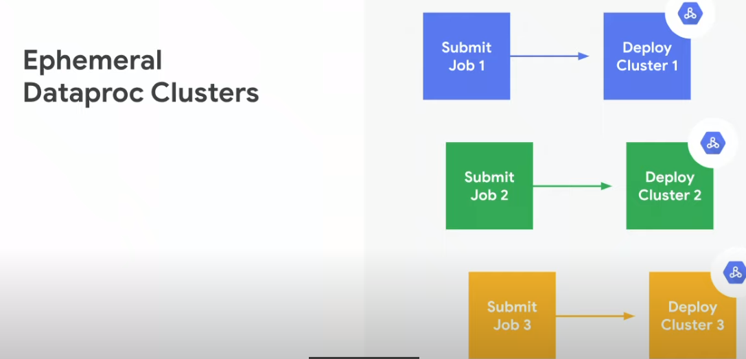
DataProc on GCP – Job Scoped Cluster Model

If your landscape is primarily ETL and Batch jobs, the job per cluster paradigm (shown below) works.

DataProc Pricing

  • Pricing consists of Cluster Size and Duration of Run

Pricing formula is: $0.010 * # of vCPUs * hourly duration

  • Dataproc clusters are billed in one-second clock-time increments
  • Scaling and autoscaling clusters. When VMs are added to the cluster, those machines are charged for the period of time that they are active. When machines are deleted, they are no longer billed.
  • Dataproc pricing is in addition to the Compute Engine per-instance pricefor each virtual machine

Basic Data Ingestion and Real Time Processing in GCP

Say you need to deploy sensor devices (e.g. Air quality measurement devices) across different cities globally.

The data to be collected from these devices should be ingested, processed and analyzed on real time basis.

The basic pipeline starts with Pub Sub.

Ingest using Pub Sub, Dump into DataFlow for pre processing and then from DataFlow, store in BigQuery, where it can be analyzed.

Need a hands-on Data Architect, AI, ML or GCP Consultant?

Need help with your data journey?  Start the conversation today.  

BigQuery Data Loading, Data Sources and Data Formats

Also read, basic data processing pipeline in GCP

Federated Data Sources for Bigquery

A Federated source (external source) is a source which allows BigQuery to query data directly without importing it in BigQuery.

DataStore is not a valid federated source.

Cloud Storage, Cloud SQL, BigTable and Google Drive are valid Data sources for federating data

Data Loading into BigQuery

While loading data into BigQuery, what if you want to allow a set percent (x % ) data to be invalid out of, say 1 million records.

You could use MaxBadRecords to specify max number of bad records.

Data Formats Supported for  BigQuery Loads

  • Batch load a set of data records from Cloud Storage or from a local file.
  • The records can be in Avro, CSV, JSON (newline delimited only), ORC, or Parquet format.
  • Proto Buffer is not a supported protocol

Need a hands-on Data Architect, AI, ML or GCP Consultant?

Need help with your data journey?  Start the conversation today.  

Delayed Sensor Data in DataFlow

Also read DataFlow Basics

Basics of Late Arriving data

Processing time is when an event is received in Dataflow. Event time can be any custom timestamp in the event e.g. event create time. Event time indicates when the event was triggered from the sensor. Due to network latency, Event time is always before the processing time.

A watermark is a threshold that indicates when Dataflow expects all of the data in a window to have arrived. If new data arrives with a timestamp that’s in the window but older than the watermark, the data is considered late data.

Apache Beam Documentation

Managing late data in DataFlow

You can allow late data by invoking the .withAllowedLateness operation when you set your PCollection‘s windowing strategy. The following code example demonstrates a windowing strategy that will allow late data up to two days after the end of a window.


PCollection<String> items = ...; 
PCollection<String> fixedWindowedItems = items.apply( Window.<String>into(FixedWindows.of(Duration.standardMinutes(1))).withAllowedLateness(Duration.standardDays(2)));

Need a hands-on Data Architect, AI, ML or GCP Consultant?

Need help with your data journey?  Start the conversation today.